Tutorial 03 – Loading and Interpreting Output#
This tutorial walks through how to load and explore Pywr-DRB simulation results using the pywrdrb.Data class.
After running a simulation (see Tutorial 02), the model writes an output file in HDF5 format containing time series data for reservoir storage, streamflows, releases, and more.
We will use the Data class to:
Load selected results sets from the
.hdf5fileInspect the structure of the results
Preview the data as pandas DataFrames
Optionally plot key results
import os
# Change to your preferred directory if needed
# os.chdir(my_directory)
cwd = os.getcwd()
print(f"Current working directory: {cwd}")
Step 1 – Specify Output Filename and Result Sets#
We begin by specifying the output file path and the results_sets we want to load. These sets tell the Data class what variables to extract from the simulation results.
Common result sets include:
'res_storage': reservoir storage (MG)'major_flow': streamflow at key nodes'res_release': combined outflow + spill at each reservoir'inflow': inflows at each catchment
A full list is available at: https://pywr-drb.github.io/Pywr-DRB/results_set_options.html
import pywrdrb

output_filename = os.path.join(cwd, "pywrdrb_output.hdf5")
datatypes = ['output']
results_sets = ['major_flow', 'res_storage']
Step 2 – Load the Output Data Using pywrdrb.Data#
The pywrdrb.Data class handles structured loading of simulation output.
Each dataset is loaded into a nested dictionary:
<results_set>is something likeres_storage<file_label>is derived from the filename (e.g.,pywrdrb_output)<scenario_index>is usually0unless running ensemble simulations
We use the .load_output() method here, since we’re loading model results.
# Initialize a data object
data = pywrdrb.Data()

# Load model output data
data.load_output(
    results_sets=results_sets,
    output_filenames=[output_filename]
    )

# Extract the dataframes for plotting
df_major_flow = data.major_flow["pywrdrb_output"][0]
df_res_storage = data.res_storage["pywrdrb_output"][0]
Step 3 – Preview Reservoir Storage#
Each column in the res_storage DataFrame corresponds to a reservoir. Each row corresponds to a simulation day.
# Preview the first few rows of storage
data.res_storage["pywrdrb_output"][0].head()
| assunpink | beltzvilleCombined | blueMarsh | cannonsville | fewalter | greenLane | hopatcong | merrillCreek | mongaupeCombined | neversink | nockamixon | ontelaunee | pepacton | prompton | shoholaMarsh | stillCreek | wallenpaupack | |
|---|---|---|---|---|---|---|---|---|---|---|---|---|---|---|---|---|---|
| 1983-10-01 | 3256.776222 | 10490.560344 | 32701.471167 | 76092.788873 | 27394.345142 | 6279.249638 | 12505.019888 | 11974.745157 | 22045.048005 | 27739.532842 | 17884.099146 | 3059.969286 | 111441.139280 | 22147.240379 | 6721.067635 | 3028.346877 | 69710.496598 |
| 1983-10-02 | 3229.674026 | 10480.779314 | 31774.993385 | 75678.636878 | 26150.691712 | 6063.296106 | 12434.655140 | 11966.924888 | 21397.929461 | 27610.869028 | 17254.298082 | 3098.192885 | 110833.521297 | 21928.605648 | 6552.604752 | 3035.271871 | 69068.486147 |
| 1983-10-03 | 3205.071202 | 10470.263708 | 30844.503718 | 75285.930854 | 24905.407834 | 5787.502806 | 12362.335673 | 11958.930889 | 20743.919708 | 27467.656487 | 16622.542298 | 3133.490218 | 110258.209023 | 21709.008357 | 6383.625397 | 3040.616105 | 68412.500014 |
| 1983-10-04 | 3165.951715 | 10459.109516 | 29911.917205 | 74761.937269 | 23658.641891 | 5480.364236 | 12289.416294 | 11950.547484 | 20082.349067 | 27276.565827 | 15990.186603 | 3167.976361 | 109490.561159 | 21488.571567 | 6214.406194 | 3045.672275 | 67735.738138 |
| 1983-10-05 | 3122.568538 | 10344.980526 | 28978.787075 | 74216.905806 | 22410.376286 | 5172.989954 | 12216.292227 | 11941.832196 | 19418.922958 | 27077.803047 | 15357.626219 | 3201.980996 | 108692.092914 | 21267.400947 | 6045.136837 | 3050.547282 | 67056.965478 |
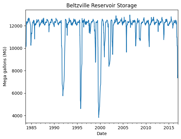
Step 4 – Plot a Time Series (Optional)#
The following example plots daily storage in one reservoir. Replace 'beltzvilleCombined' with any reservoir name from the DataFrame.
import matplotlib.pyplot as plt

df = data.res_storage["pywrdrb_output"][0]
df["beltzvilleCombined"].plot(title="Beltzville Reservoir Storage")
plt.ylabel("Mega gallons (MG)")
plt.xlabel("Date")
plt.show()
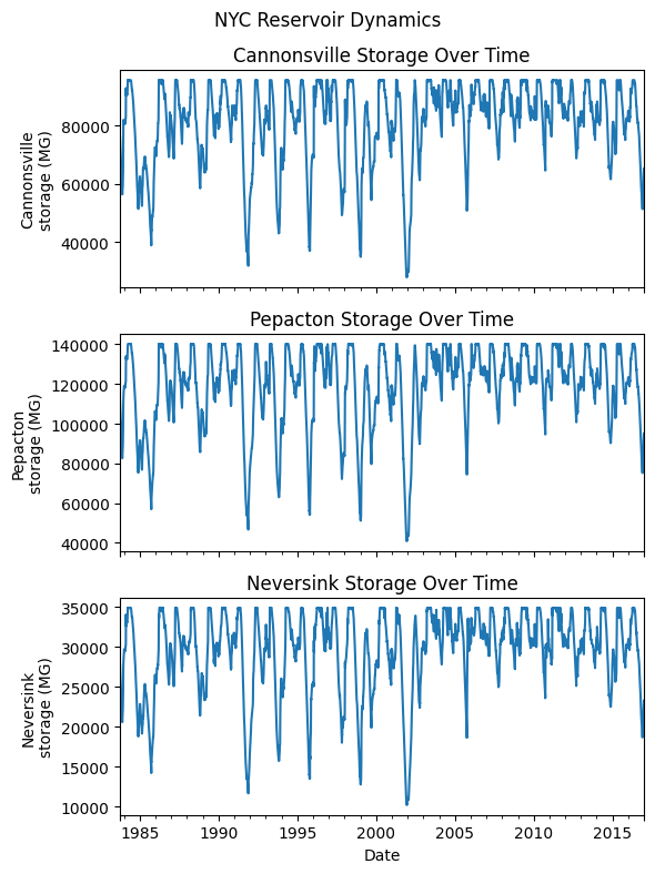
Exploring NYC Reservoir Dynamics#
Pywr-DRB includes a detailed representation of the New York City (NYC) reservoirs, which play a critical role in supplying water to downstream users and managing drought risk in the Delaware River Basin.
The three major NYC reservoirs are:
Cannonsville
Pepacton
Neversink
By visualizing their simulated storage dynamics, we can assess seasonal variability, drought resilience, and management impacts over time.
# Define NYC reservoirs to plot
nyc_reservoirs = ['cannonsville', 'pepacton', 'neversink']

# Create subplots
fig, axes = plt.subplots(nrows=3, ncols=1, figsize=(6, 8), sharex=True)

for ax, res in zip(axes, nyc_reservoirs):
    df_res_storage[res].plot(ax=ax)
    ax.set_ylabel(f"{res.capitalize()}\nstorage (MG)")
    ax.set_title(f"{res.capitalize()} Storage Over Time")

plt.xlabel("Date")
plt.suptitle("NYC Reservoir Dynamics", y=0.98)
plt.tight_layout()
plt.show()
Summary#
You’ve now loaded and explored results from a Pywr-DRB simulation.
You can use these outputs for further analysis, visualization, or calibration diagnostics.
The
Dataclass ensures consistency when working across observed data, simulated outputs, and hydrologic model flows.
Next Step:#
Move to Tutorial 04 – Using Custom Input Data to simulate using your own inflow, release, or storage files.